Inferring Concept Drift Without Labeled Data

FF22 · ©2021 Cloudera, Inc. All rights reserved

This is an applied research report by Cloudera Fast Forward Labs. We write reports about emerging technologies, and conduct experiments to explore what’s possible. Read our full report about Inferring Concept Drift Without Labeled Data below, or download the PDF. You can view and download the code accompanying our concept drift experiments on Github.

Introduction

After iterations of development and testing, deploying a well-fit machine learning model often feels like the final hurdle for an eager data science team. In practice, however, a trained model is never final. This milestone marks just the beginning of the perpetual maintenance race that is production machine learning. This is because most machine learning models are static, but the world we live in is dynamic. More specifically, the ability of a trained model to generalize relies on an important assumption of stationarity - meaning the data upon which a model is trained and tested are independent and identically distributed (i.i.d). In real-world environments, this assumption is often violated, as human behavior - and consequently the systems we aim to model - are dynamically changing all the time.^[1]

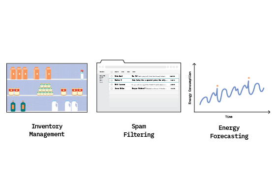
Take, for instance, the impact of the COVID-19 pandemic on algorithm-driven businesses like inventory management. Instacart’s model for forecasting in-store product availability dropped from 93% to 61% accuracy, due to a drastic change in shopping behavior as consumers stockpiled what previously were infrequently purchased goods. The model was forced to adapt to this transitory shift in its prior understanding of the world.

Not all changes are this sudden, though. Consider the task of maintaining an email spam filtering service. The core technology consists of a text classification model that picks up on keywords in email content to block spammers. Over time, users will begin to manually report more messages as spam that are not caught by the filter. In this adversarial environment, spammers are continuously adjusting terminology to outwit the deployed spam filters, so models must relearn what language constitutes the evolving concept of spam to remain effective.

Or think about the job of forecasting energy consumption, in which historical demand is just one piece of the puzzle. In practice, future demand is driven by a slew of non-stationary forces - like climate fluctuations, population growth, or disruptive clean energy tech - that necessitate both gradual and sudden domain adaptation.

Changes in environmental conditions like these are referred to as concept drift, and will cause the predictive performance of a model to degrade over time, eventually making it obsolete for the task it was initially intended to solve.

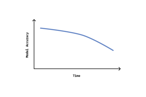
To combat this divergence between static models and dynamic environments, teams often adopt an adaptive learning strategy that is triggered by the detection of a drifting concept. Supervised drift detection is generally achieved by monitoring a performance metric of interest (such as accuracy) and alerting a retraining pipeline when the metric falls below some designated threshold.

While this strategy proves to be effective in theory, there are several limitations that often prevent its use in practice. Namely, it requires immediate access to an abundance of labels at inference time to quantify a change in system performance - a requirement that may be cost-prohibitive, or even outright impossible, in many real-world machine learning applications.

In this report, we explore broadly applicable approaches for dealing with concept drift when labeled data is not readily accessible. We’ll start by defining what we mean by concept drift and frame the limitations of supervised methods for detecting it. Then, we’ll discuss why true unsupervised concept drift detection is not possible, and explore several alternative methods for dealing with it. Finally, we’ll share the results of our experiments with the proposed methods, and wrap up with a discussion of considerations and limitations.

Background

What is concept drift?

Most machine learning systems today operate in a batch paradigm; they probe a historical data set to develop a model that reflects the world as it was at the time of training. But, as we’ve seen, the world is always changing, and the complex relationships that a model abstracts are also likely to change over time - causing model performance to deteriorate, if not accounted for. This phenomenon in which the statistical properties of a target domain change over time is considered concept drift.^[3]

Formally, concept drift between time \(t\) and \(t+1\) can be defined as:

$$P_{t}(X,y) \not= P_{t+1}(X,y)$$

where \(P_t\) denotes the joint probability distribution at time \(t\) between the set of input variables \(X\) and the target variable \(y\). Since the joint probability can be decomposed as the product of the probability of \(X\) and the conditional probability of \(y\) given \(X\), changes in a data stream can therefore be characterized by changes in the components of this relationship according to the equation below.

$$P_t(X,y) = P_t(X) \times P_t(y|X)$$

This decomposition yields two underlying sources of drift - feature drift and real concept drift.

Source 1: Feature Drift

Feature drift (also referred to as covariate shift, feature change, input drift) characterizes the scenario where the distribution of one or more input variables change over time (i.e., \(P(X)\) changes).

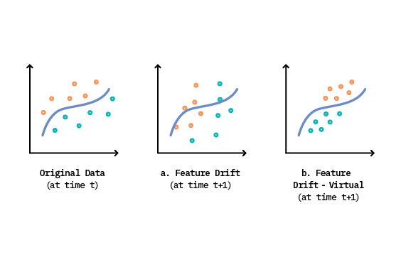
This is seen in both Figure 3.a & 3.b above, where the distribution of features has changed from time \(t\). In Figure 3.a, feature drift has occurred in a region that directly affects the outcome of the learned classification boundary, causing model performance to decrease (and thus making it classified as both feature drift and real concept drift). However, feature drift can also occur where \(P(X)\) changes over time, but the changes do not affect the learned decision boundary. This describes a specific type of feature drift called virtual drift, as seen in Figure 3.b. This is an important distinction because, as we see here, only the changes in \(P(X)\) that affect the prediction decision actually warrant a model adaptation.

For example, consider a clothing brand that is looking to recommend items for a given customer as relevant or not relevant. Suppose this customer lives in a tropical climate. Lightweight, breathable clothing items are relevant to them - while heavy, cold weather apparel is not. In this scenario, the independent features \(X\) are both the customer’s preferences (e.g., age, size, location) and the brand’s product line. The dependent variable, \(y\), is the relevance of a clothing item to the customer.

If the brand’s lead designer quits and is replaced, the brand’s design style will naturally change as a result (i.e., change in \(P(X)\)). However, warm weather clothing still remains relevant for this customer, despite the stylistic differences (i.e., no change in \(P(y|X)\)). This scenario corresponds to a virtual drift.^[4]

Suppose now that, due to a shift in brand strategy, the company alters their product focus to sell mostly cold weather gear and fewer warm weather items, but the designer (and style) stay the same. This scenario also corresponds to a feature drift (Source 1); however, it’s one that does impact the decision boundary (i.e., \(P(y|X)\)). Therefore, this scenario is also categorized as Source 2 drift.

Source 2: Real Concept Drift

The second source of drift, called real concept drift (also commonly referred to as actual drift, concept shift, conditional change), refers to changes in \(P(y|X)\) and signals that a previously learned relationship between features and targets no longer holds true. Unlike feature drift, this type of drift will always cause a drop in model performance.

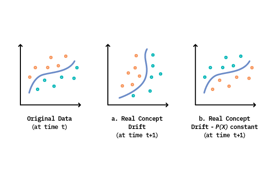
It’s important to note that real concept drift can happen either with or without a change in \(P(X)\).^[5] This nuance is shown in Figure 4.a, where both the input feature distributions and the learned decision boundary have changed in the new time step. In contrast, Figure 4.b demonstrates a scenario where input distributions remain constant, while the ground truth class labels have actually evolved.

Continuing with our previous example, suppose that the customer moves from their tropical paradise to the Alaskan tundra, while the clothing brand makes no changes to their offerings or staff. In this case, the very meaning of “relevance” flips, making cold weather gear relevant and warm weather clothing irrelevant. This describes another example of real concept drift, but with no change in \(P(X)\).

However, the real world is rarely ever this clean-cut, and oftentimes both sources of drift are at play simultaneously. Let’s now imagine a situation where the customer moves to a temperate climate with cold nights and warm days, and the company slightly alters their product mix towards cold weather gear. Here, we observe changes in both \(P(X)\) and \(P(y|X)\), making it difficult to attribute concept drift to any single source.

What is a data stream?

Before moving on, let’s define some additional terminology that will be mentioned throughout this report. To discuss the idea of concept drift in production, we must consider dynamic data environments. For this reason, we reference concept drift detection and adaptation with regard to data streams, where instances arrive continuously and sequentially over time. Streaming data is often generated on the fly - potentially at a fast and variable rate, and with infinite range - making it a prime candidate for evolving data distributions.

Despite this, concept drift is not exclusive to data streams. And, in order to frame a discussion involving both stream and batch contexts, concept drift detection methods commonly employ the notion of sliding windows, or groups of sequentially ordered observations.

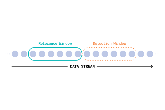
In general, one window contains the instances belonging to the most recent known concept, which were used to train or update the deployed model, and one window contains instances which may have suffered a concept drift. We refer to these windows as the reference window and detection window, respectively.^[6]

Framing the problem

With these definitions in mind, we see that real concept drift in a data stream (Source 2) poses the main concern for production models, since it directly impacts model performance. The most effective solution to address this issue involves detecting when the learned relationship between features and targets is no longer appropriate for incoming data, and then training a new model to learn the novel concept. An adaptive workflow like this is shared among common supervised methods like Drift Detection Method (DDM), Early Drift Detection Method (EDDM), and ADaptive WINdowing (ADWIN). We describe this workflow in Figure 6, below.

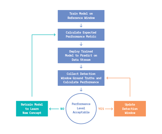
In general, these techniques monitor a task-dependent performance metric like accuracy, F-score, or precision/recall. If the metric of interest deviates from an acceptable level (as determined during training evaluation on the reference window), a drift is signaled.

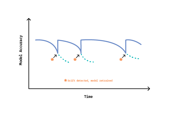
The cumulative effect of this approach over the lifetime of a machine learning system is highlighted in Figure 7. Initially, the system celebrates strong performance because the model has learned from recent data. After some time, accuracy declines as concepts evolve, until ultimately a metric threshold is crossed, and drift is detected. System performance then realizes an immediate boost after retraining, as the new concept is absorbed.

Despite the ample research and proven effectiveness of these supervised methods, they all suffer from a shared, impractical assumption － that true labels are instantaneously available after inference. In most use cases, the immediate availability of true labels is infeasible for several reasons.

First, annotating data is expensive, in both cost and labor, as it often requires hired domain expertise. The issue is described succinctly by the authors of On the Reliable Detection of Concept Drift from Streaming Unlabeled Data:

“To highlight the problem of label dependence, consider the task of detecting hate speech from live tweets, using a classification system facing the Twitter stream (estimated at 500M daily tweets). If 0.5% of the tweets are requested to be labeled, using crowdsourcing websites such as Amazon’s Mechanical Turk2, this would imply a daily expenditure of $50K (each worker paid $1 for 50 tweets), and a continuous availability of 350 crowdsourced workers (assuming each can label 10 tweets per minute, and work for 12 hours/day), every single day, for this particular task alone. The scale and velocity of modern day data applications makes such dependence on labeled data a practical and economic limitation.”

Second, in addition to label scarcity, verification latency - or the period between the availability of an unlabeled test instance and the availability of its true label - is application-dependent and often variable.^[7] For example, it can take several months for an act of credit card fraud to be reported (i.e., ground truth) from the time the fraudulent transaction occurred. If F1 score is the only metric being used to track model performance (and thus detect concept drift), there may be several months of higher than normal fraudulent activity without any signal that something is wrong.

Finally, some use cases operate in an extreme case of infinite verification latency, where ground truth labels are impossible to ever obtain. Consider a bank which uses machine learning to power its lending decisions. If a model predicts a loan will default for a given applicant, the loan is never granted; therefore, it can never be determined if the loan would have actually defaulted or been repaid. Use cases like this demand an alternative solution.

Addressing the problem

Due to these limitations, there is a clear need for effective methods that can detect real concept drift (Source 2) in an unsupervised manner. Unfortunately, this proves to be an impossible task, as the only way to confirm a change in \(P(y|X)\) with certainty is to have some access to ground truth labels - there is no free lunch.

In the absence of labeled data, the best we can do is attempt to infer real concept drift by detecting feature drift (Source 1). That is, we are interested in quantifying visible changes in \(P(X)\) and surmising that those changes correspond to meaningful change in the classification boundary \(P(y|X)\). Of course, this approach is prone to error because as we’ve seen:

1. Not all changes in \(P(y|X)\) are visible from \(P(X)\), resulting in false negative detections where real drift occurs but is not signaled.
2. Not all changes in \(P(X)\) actually affect \(P(y|X)\), resulting in overly sensitive detectors that trigger costly false positive detections.

Inferring real concept drift in an unsupervised fashion thus becomes a delicate balancing act, in order to minimize the number of false positive detections (and therefore labels needed) while remaining sensitive enough to pick up on meaningful changes in the feature space that likely contribute to a change in concept.

Methods for inferring concept drift

In comparison to recent research on supervised drift detectors, much less attention has been paid to unsupervised methods.^[8] However, detecting shifts in data distributions is a well-explored field of data mining, with solutions ranging from multiple hypothesis testing and novelty detection to discriminative distance and algorithm-specific techniques. In our exploration, we focused on methods that are model-agnostic and truly unsupervised, to ensure broad applicability in practice. In this section, we present four methods for inferring concept drift without labels, and use a binary classification task to frame the discussion.

1. Statistical test for change in feature space

The ultimate goal of feature drift detection is to determine if two distributions are different. Therefore, the first and most basic approach to infer concept drift applies a hypothesis test to flag if a statistically significant change has occurred between the reference and detection windows for each feature in a given data stream.

For continuous features, we use a two-sample Kolmogorov-Smirnov (KS) test, which is a non-parametric hypothesis test used to check whether two samples originate from the same distribution. For categorical features, we make use of a Chi-Squared goodness of fit test.

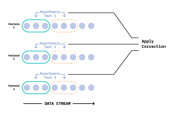
In the case of multivariate tabular data, we can test each feature independently (while accounting for multiple tests) to arrive at an overall signal of drift or no-drift, as seen in Figure 8. The Bonferroni test is a notable approach for correcting multiple hypothesis tests - while making conservative assumptions about the (in)dependence among them - to arrive at a final result.

In contrast to this feature-wise approach, we could also apply a multivariate two-sample hypothesis test like the kernel-based technique called Maximum Mean Discrepancy (MMD). MMD allows us to distinguish between two probability distributions, based on the mean embeddings of those distributions. While this method does side-step the need for multiple tests, the choice of kernel is critical to ensuring its correctness, and a linear time complexity imposes a potential bottleneck in streaming applications.^[9]

While feature-wise and multivariate hypothesis testing is broadly applicable across machine learning use cases, it has several limitations as a real concept drift inference tool. Because these methods consider drift in each feature to be equally important (despite p-value correction across tests), they are prone to false positive detections. Imagine the case where several features in a datastream exhibit drift, but none of them are of high importance to a classifier’s decision-making process. It’s likely that the present drift will not actually impact the learned decision boundary, despite the hypothesis test’s ringing alarm.

This limitation arises because we’ve excluded the classifier from the detection process and are making decisions solely on the distribution characteristics of incoming features - resulting in increased sensitivity to change and a high number of false alarms.

2. Statistical test for change in response variable

Unlike the previous method, where only the feature space is analyzed, our second approach infers concept drift by tacitly involving the classifier in the detection process, making change detection relevant to the prediction task at hand. To do so, we apply a model that’s been trained on the reference window to generate predicted class probabilities (a response distribution) for observations in the detection window. Then, we use a k-fold procedure to obtain probability estimates for the reference window.

With our two populations in hand, we can apply a Kolmogorov-Smirnov hypothesis test to see if the response distributions between reference and detection windows differ significantly. In effect, the trained model serves as a dimensionality-reducing preprocessing step. It leverages its learned relationship between features and targets (i.e., \(P(y|X)\)) to generate a response distribution that is sensitive to feature space changes that will likely affect the performance of the model in question. If important features in the detection window have drifted from those the model learned on, we would expect the classifier to produce significantly different response distributions, as depicted in Figure 9.

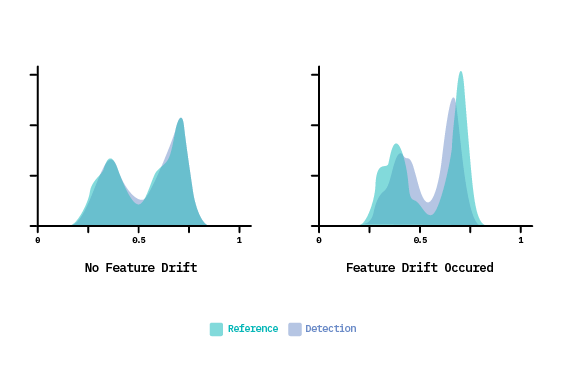
Although it’s a step in the right direction, this method is still overly sensitive. That’s because, by design, a KS test is responsive to changes across the entire response distribution. But do we really care about changes in regions of high confidence? For example, if the density shape between 0 and 0.25 confidence level changes a bit, it doesn’t impact the classification outcome of those points, because they’re still well below the 0.5 decision threshold. This leads us to the next approach.

3. Statistical test for change in margin density of response variable

Rather than test for changes across the entire cumulative response distribution, we can instead focus on just the regions of uncertainty around our decision threshold, where slight variations in confidence lead to different classification outcomes.

To do so, we must introduce a parameter that specifies a desired margin width around the decision boundary, to define a region of uncertainty. Margin here is the portion of the prediction space which is most vulnerable to misclassification.^[12] Then, for both windows, we classify each observation as in-margin or out-of-margin, based on its predicted confidence score. We compare these categorical populations between windows, using a Chi-square goodness of fit test to check for significant changes in the margin density. The underlying assumption here is that a significant change in the number of samples in the margin is indicative of a drifting concept.

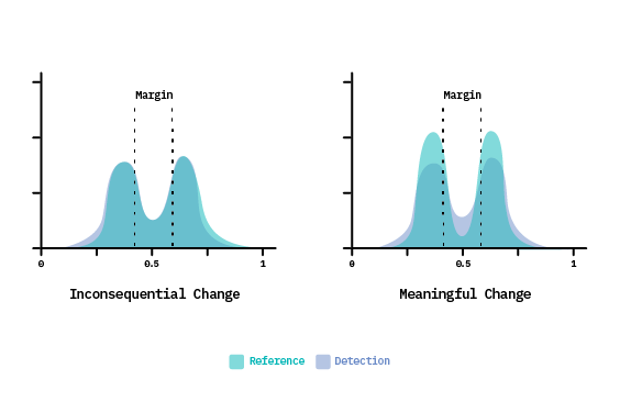
The impact of this approach is highlighted in Figure 10, above. On the left, we see the case where a divergence exists towards the tail ends of the distribution, but the rest of the probability space remains congruent. This example would fail the KS test (described in Method 2), signaling a feature drift, and consequently request costly new labels for retraining. However, because the divergence exists far from the decision boundary, it would likely not have impacted the classification results, making it a false positive detection. In contrast, the margin density approach would tolerate this inconsequential change. Only when a statistically significant divergence occurs inside the margin will Method 3 raise an alarm, as shown in Figure 10 (on the right).

Introducing a margin of uncertainty to desensitize feature drift detection does help reduce the number of false positive detections. However, there is still room for improvement. Each method we have discussed so far relies on hypothesis testing to signal drift. Unfortunately, the mere falsity of a null hypothesis doesn’t say much about our window samples, other than that they don’t come from an identical population. But do we really care if the populations are identical?

If our goal is to reduce the sensitivity of feature drift detections, we probably care more about quantifying how different two populations are, which is something that a statistical test cannot provide. A quantitative measure of similarity affords us the flexibility to set our own threshold, depending on our tolerance for error. In essence, we need a way to distinguish what level of change is statistically significant from what is practically significant.

4. Detect change in margin density of response distribution using a learned threshold

Our final method uses a learned threshold to detect change in the margin density of a response distribution. Building upon the previous two methods, we first obtain a response distribution for each window, and introduce a margin to classify predictions as in or out of the region of uncertainty. However, rather than applying a Chi-square test (as in Method 3), we establish an expected value for margin density based on the reference window.

This is accomplished during the k-fold procedure by calculating the percentage of instances falling in margin, relative to the total instances in the window (i.e., margin density) for each fold. The cross-validation procedure produces a population of \(k\) margin density values from which we can calculate a mean (\(MD_{ref}\)) and standard deviation (\(\sigma_{ref}\)), providing a strong estimate of the expected margin density value and an acceptable deviation.

These values are then used to signal change in the detection window based on a desired level of sensitivity, \(S\). A practically significant change is signaled when the margin density of the detection window differs by more than \(S\) standard deviations from the expected margin density value, as seen in the equation below.

$$ |MD_{det} - MD_{ref}| > S \times \sigma_{ref} $$

By setting the expected margin density value from the population observed in the reference window, we establish a baseline specific to the problem at hand. Adding the sensitivity parameter offers control over the detection process. Larger values of \(S\) will reduce the number of false positive detections, but possibly at the cost of increasing false negatives - a decision that might make sense when the cost/impact of a false negative is low. Inversely, lowering \(S\) might be a good idea for critical applications, where the cost of a real drift could be harmful if undetected.^[13]

Experiments

To gain a deeper understanding of these unsupervised concept drift detection methods, we needed to experiment. In particular, we aimed to understand the tradeoff between false positive and false negative drift detections produced by each of these methods over a machine learning system’s lifetime. To do so, we designed an experimental setup - which consisted of an adaptive learning workflow with a synthetic dataset - to simulate the lifecycle of a model in production.

Inducing concept drift

Experimenting on production-related issues like concept drift is challenging. Concept drift research is often performed on purely synthetic datasets, where variables are randomly generated according to predefined rules to allow for control over the type, timing, and magnitude of drift. However, these datasets do not truly mimic the relationships present in real world data. In contrast, real world datasets lack precise flags for the start and end of drifting concepts and often include mixed drift types, making it difficult to cleanly evaluate drift detection methods.

For our experimentation, we decided to induce drift into a real dataset, as it allowed us to retain genuine data properties while ensuring significant drift was actually present. To do so, we applied an extended version of the drift induction process that was used by the authors of On the Reliable Detection of Concept Drift from Streaming Unlabeled Data to the Covertype Data Set from the UCI Machine Learning Repository​. Before inducing drift, the dataset was reduced to a binary classification problem, by considering only the two most populous classes, and all features were normalized in the range of [0,1]. Additionally, all soil type variables were dropped, to simplify the problem. This resulted in a dataset with 14 features, one binary target variable, and ~495,000 observations.

The drift induction process works by first shuffling the entire dataset in an attempt to remove any existing concept drift. We then create changepoints in the data stream, by selecting a subset of features and randomly rotating their values for all examples after a given changepoint (the equivalent of randomly swapping columns). This basic approach ensures that feature drifts are induced, while also maintaining the original properties of the dataset.

We created three changepoints evenly spaced across the entire dataset. For the first changepoint, we selected the three most impactful features to rotate (determined by ranking features based on their impurity-based feature importance). For the second changepoint, we selected the fourth to tenth most important ranked features to rotate. And finally, we selected the remaining three least important features for the third changepoint. At each changepoint, drift was forward chained through the remainder of the dataset to provide consistency across concepts. This process resulted in four unique “concepts” (~124k observations each) with varying degrees of drift. The entire data preparation and drift induction process we followed can be referenced in this notebook.

Experimental Setup

With a drifting dataset in hand, we then implemented a rudimentary adaptive learning workflow, in order to evaluate the proposed detection methods (discussed above) in a lifecycle context. The workflow consisted of two sliding windows (reference and detection) of fixed size passing over the drift induced datastream, where the decision to retrain at each timestep is made by the given drift detection method.

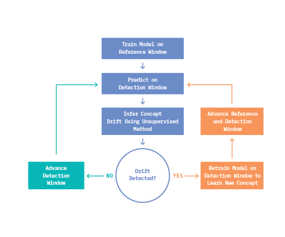
The workflow described in Figure 11 ran until predictions were generated for every observation in the data set. Throughout each experiment, we recorded the incremental accuracy of predictions on the datastream, as well as the number of requested true labels. Incremental accuracy provides a cumulative measure of performance of the classification system over the entire datastream, since several different “deployed” models likely exist. The number of requested true labels corresponds directly to the number of drift detections, and thus to the number of retrainings demanded.

In addition to accuracy and number of retrainings, we also captured if a real concept drift occurred at each window timestep (irrespective of what the drift detection method indicates). Of course, this is a luxury we are only afforded in an experimental setting because we have access to all ground truth labels, which allows us to evaluate our various drift detection methods. This source of truth is determined using a k-fold approach on the reference window, similar to that used in Method 4 above, except rather than gathering a population of k margin density values, we collect a population of accuracy measures to establish an expected accuracy and acceptable deviation. If the accuracy on the detection window falls outside three standard deviations of the expected accuracy, we conclude that a real concept drift occurred (i.e., significant change in \(P(y|X)\)). This approach for quantifying real concept drift (versus just using the three drift induced changepoints) allows us to account for unknown drifts that may exist in the underlying data, despite our attempt at removing it via random shuffle. This ground truth indicator serves as the basis for classifying drift detections as false positives or false negatives.

Using this experimental setup, we evaluated detection methods 2, 3, and 4 from above. We compared the results against a baseline and topline scenario. The baseline case is simply a classifier that never adapts to drift (i.e., it is trained only on the initial reference window and used to evaluate on the entire remaining datastream). The topline scenario greedily retrains a new model at each window timestep.

All our experiments shared a common set of parameters - including model type (random forest classifier), model hyperparameters (n_estimators=5, max_depth=5) , and window size (35,000 observations). The window size and model hyperparameters were empirically selected by finding a combination that did not result in overfitting between reference and detection sets, while allowing multiple window timesteps to fit within each induced concept. Our entire set of experiments and supporting code can be found here.

Results

The cumulative accuracy of each drift detection experiment is visualized and summarized over the full datastream in Figure 12, below. Here, the vertical lines represent the equally spaced changepoints where drift was systematically induced in the datastream.

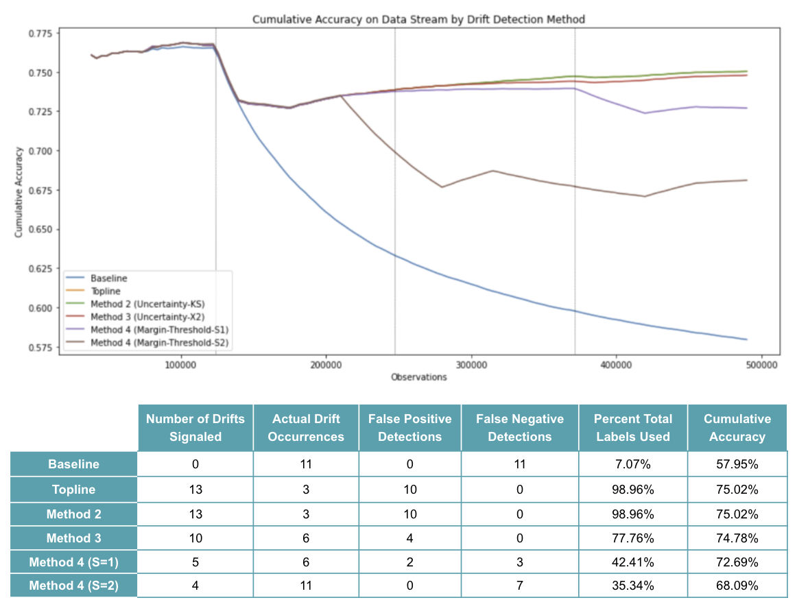
By observing the baseline case (blue line) where no model retraining occurs after the first window, we see a steep decline in accuracy immediately after the first changepoint. This makes sense because the changepoint introduces a severe drift (i.e., rotation of most important features) and, without adaptation, the model fails to reflect the new concepts - resulting in a drop of ~18% accuracy from initial training to the end of the data stream.

In contrast, we see that by retraining at each window timestep, the topline case (orange line overlapping with green line) is able to recover from each concept change, resulting in a cumulative accuracy drop of just ~2% over the datastream. Of course, this comes at the cost of 13 retrainings (or 99% of the total labels requested) where only three actually experienced concept drift. This results in 10 false positives.

As mentioned above, we see that Method 2 (KS test on response distribution) produces identical results to our topline case; the test signals a drift at every window timestep. Intuitively, this does not make sense, because there are three distinct windows (of 35,000 records each) within each induced concept - that is, three opportunities for the model to learn and adapt to each new concept. This points to the major flaw of Method 2: comparing entire response distributions with a KS test proves to be overly sensitive to small differences that may actually be deemed acceptable in practice (thus prompting a request for unnecessary retraining).

This is further evidenced by observing the results for Method 3 (Chi-squared test on response margin) where only 10 drifts were signaled - while still capturing all six actual drift occurrences, but still producing four false positive detections. In this case, by statistically testing for significant changes inside of a defined margin vs. the entire distribution, we required just 77% of the total labels while maintaining a cumulative accuracy within 1% point of the topline case, and did not sacrifice any false negative (missed) detections.

Finally, we see that Method 4 (using a learned threshold of margin density) relaxes drift detections even further. With the sensitivity value set to one, we observe only five drift detections demanding just 42% of the total labels, while producing a cumulative accuracy just 2% points lower than the topline case. However, by stepping away from statistical tests, we notice that this experiment actually misses three windows of actual drift (false negatives). Increasing the sensitivity parameter to a value of two exacerbates this problem, decreasing the cumulative accuracy even further, as seven actual drift occurrences are missed.

Limitations

As mentioned previously, experimenting with concept drift is challenging, because it requires us to simulate a production environment and make assumptions in an attempt to emulate it. One assumption that we made while designing our dataset is that randomly shuffling all records upfront would eliminate existing drift and provide a clean slate upon which we could introduce controlled drift. This false assumption was brought to light as we saw more than three actual drift occurrences in several of the experiments. Because we chose to define real drifts by comparing change in accuracy between reference and detection windows, we saw an unequal number of “actual drifts” across experiments, making head-to-head comparison of results difficult.

Additionally, we chose to implement non-overlapping, fixed-size windows that advance in full for all experiments. Many drift detection methods today operate in an incremental or online fashion where detection windows are advanced for each incoming observation rather than batches. This strategy eliminates the period of inactivity until a new detection window reaches the minimum number of samples, and may decrease the delay in response time for sudden drift detections.

Another limitation is seen in our rudimentary retraining scheme, where labels are requested for the entire detection window upon a drift signal and the existing model architecture is retrained in place. In practice, there are a variety of retraining options - like using all available historical data, weighting newer observations, dropping outdated records, or requesting just a portion of labels from the newest window. In addition, naive retraining of the same model with new data might not be enough to adapt to an evolved concept.^[14] A manually selected model architecture may perform better upon each retraining, which points to another limiting assumption of our experimental setup.

Considerations

So far we have discussed and experimented with approaches for dealing with concept drift when the ground truth of the newly available data instances isn’t readily available. While we covered methods that are model agnostic and truly unsupervised, detecting concept drift in practice is not a straightforward task. As noted by the researchers of Learning under Concept Drift: A Review, handling concept drift is generally coupled with other machine learning problems. In this section, we cover a few of these overlapping issues along with some considerations when designing a drift detection strategy.

Ethics

It’s impossible to design a machine learning system and know everything about the domain upfront. As we’ve seen, concept drift occurs by default, as a result of static models operating in dynamic environments. Therefore, deployed models will naturally have unintended consequences. For this reason, it’s imperative that teams plan for uncertainty post-deployment and establish robust monitoring and detection processes , so as to understand when something has gone wrong and take corrective action.

However, the act of monitoring a feature or metric just to “check the box” is not enough. Blindly optimizing and maintaining a poorly selected set of metrics will result in far from optimal outcomes. This is because metric optimization often leads to manipulation, gaming, and a focus on short-term quantities at the expense of longer-term concerns. When developing a post-production strategy, it’s important to use a slate of metrics to gain a fuller picture of a model’s true impact, combine metrics with qualitative accounts, and involve a range of stakeholders - including those who will be impacted downstream by the model’s decisions.^[15] Planning for and monitoring a model’s impact on a wider set of concerns than just predictive performance adds an additional layer of complexity to the already difficult task of production machine learning - but it’s a requirement, not an option.

Other Prediction Tasks

Up until now, all of the methods discussed for inferring drift have been in the context of binary classification. But how can these approaches be extended to other tasks, like multiclass classification and regression?

At the core of our approaches, we are simply using a trained model to produce a distribution of uncertainty and then comparing that distribution between reference and detection windows. Therefore, we can apply this same idea to other tasks by reformulating our definition of uncertainty. In the binary classification task, uncertainty exists as the difference between the two class probabilities. In a multiclass classification task, uncertainty could be defined as the difference between the top two class probabilities. Similarly, for regression tasks, the notion of uncertainty could take the form of absolute error of each prediction.

Class Imbalance

The common issue of class imbalance is exacerbated when it comes to drift detection. Class imbalance occurs when the proportion of data instances belonging to each class varies, causing certain classes to be underrepresented. It is usually the underrepresented classes in such situations that end up having higher misclassifications. Detecting drift between populations with imbalanced classes is complicated, and becomes more challenging when the data between windows cannot be stored due to memory issues. As such, approaches that cater to both concept drift and class imbalance in data streams are relatively less studied.^[16] That said, CDS (Concept Drift with SMOTE (Synthetic Minority class Oversampling Technique)) is one of the more recent batch-based incremental learning algorithms that strategically uses the minority class data to tackle this problem.^[17]

Another related problem that is largely underexplored is dealing with multi-label classification, where a particular data instance could be associated with one or more labels. For example, a news article may have overlapping classes like “politics,” “environment,” and “energy.” Multi-label data streams contain independent relationships for each label - where each concept is likely to have its own drift pattern that may drift asynchronously from its peers. In addition, label proportions may not be consistent across detection windows. To address these challenges, a notable approach^[18] associates each label with two fixed size instance-windows, one for positive examples and the other for negative examples for the training data. The size of the positive window is a user-specified parameter, and it should be large enough to learn an accurate model, but small enough to reduce the probability of drift within the window. The number of negative examples in the negative window is determined based on the ratio of the number of positive examples to another user-specified parameter: distribution ratio. This parameter plays the role of balancing the distribution of positive and negative examples in the union of the two windows and ranges typically from 0.3 to 0.7. The approach allows it to oversample the positive and undersample the negative examples for all labels. They further build and use k-nearest neighbor (k-NN) classifiers to determine the label of an unlabeled test instance. Normally a k-NN classifier outputs a class label based on whether the probability of it belonging to the positive class is >= 0.5. This default behavior is an improper choice when it comes to imbalanced classes, and the authors instead propose a batch-specific thresholding approach to combat that.

Active Learning

Active learning is a set of machine learning techniques that reduces the number of labeled examples required to train a model. In settings where the labeled examples are available only initially or are scarce, active learning approaches utilize these labels to build an initial model, and then uses this model to request labels for data points (from a human) that the model finds hard to predict on. A scenario where the unlabeled data stream is drifting could pose additional challenges. For instance, active learning strategies that request labels for the most uncertain instances would typically concentrate around the decision boundary. Changes that occur further from the boundary may be missed, and models may fail to adapt. Some solutions to effectively tackle such challenges include learning strategies that are guided by drift detection to save labeling costs for difficult and evolving instances.^[19][20]

Semi-supervised Learning

Semi-supervised and transductive learning techniques leverage both labeled and unlabeled examples to learn more generalized models when limited labeled data is available for training. Because this technique naturally learns from unlabeled data, it may be assumed that models of this type can easily track drifting concepts. That is not the case, however, because with concept drift, training data and test data are generated from different underlying distributions. Due to this unique learning paradigm, there have been many new developments specific to semi-supervised and transductive learning in the presence of concept drift. For instance, the weight estimation algorithm (an ensemble-based classifier approach^[21]) uses unlabeled test data along with a set of mixture models to adjust classifier voting weights. The approach helps detect gradual or incremental drifts. There is also the COMPOSE (COMPacted Object Sample Extraction) approach, which can handle multi-class data, including the scenario of new classes or new subpopulations for gradual drift detection.^[22])

Big Data

Data in big data streaming environments is often generated at a fast rate in large quantities, and is highly volatile - a scenario prime for drifting concepts. Due to the high throughput nature, it may not always be feasible to capture, store, and process all the data. This complication has led to the development of scalable and parallel algorithmic implementations that only need one pass through the data, and thus train and adapt to concept drifts in real-time scenarios. For instance, the Online MapReduce Drift Detection Method (OMR-DDM)^[23]) detects drift by the use of the error rate of a collection of classifiers executed concurrently. Approaches like Micro-Cluster Nearest Neighbor (MC-NN)^[24]) do not need data to reside in memory, are processed incrementally, and adapt to concept drifts by monitoring classification error.

Conclusion

As we’ve learned, maintaining a static representation of an ever-changing environment is challenging, and requires diligent performance monitoring to signal when a machine learning model is no longer suited for its original task. This issue becomes even more difficult when the cost or availability of ground truth labels make performance-based drift detection methods infeasible － which is often the case in real world applications.

In this scenario, teams must monitor and detect changes purely from independent variables as a means to infer concept drift. Unfortunately, monitoring changes in input distributions produces many false positive detections, because not all changes in the feature space of a population actually correspond to a meaningful drift in relation to the target variable.

In this report, we presented four ways to infer concept drift in an unsupervised manner, with the goal of reducing false positive drift detections. We reported experimental results comparing and contrasting the nuances of each method, and conclude that the best approach for detecting drift without labels will depend on your specific application’s tolerance for error.

We hope this report has brought to light a few practical challenges associated with production machine learning, and we look forward to continued research in this space!

---

1. On the Reliable Detection of Concept Drift from Streaming Unlabeled Data ↩︎

2. Domain adaptation ↩︎

3. Learning under Concept Drift: A Review ↩︎

4. A Survey on Concept Drift Adaptation ↩︎

5. A Survey on Concept Drift Adaptation ↩︎

6. An overview of unsupervised drift detection methods ↩︎

7. Fast Unsupervised Online Drift Detection Using Incremental Kolmogorov-Smirnov Test ↩︎

8. An overview of unsupervised drift detection methods ↩︎

9. Optimal kernel choice for large-scale two-sample tests ↩︎

10. Failing Loudly: An Empirical Study of Methods for Detecting Dataset Shift ↩︎

11. On the Reliable Detection of Concept Drift from Streaming Unlabeled Data ↩︎

12. On the Reliable Detection of Concept Drift from Streaming Unlabeled Data ↩︎

13. On the Reliable Detection of Concept Drift from Streaming Unlabeled Data ↩︎

14. Machine Learning Monitoring, Part 5: Why You Should Care About Data and Concept Drift ↩︎

15. Reliance on Metrics is a Fundamental Challenge for AI ↩︎

16. Incremental learning imbalanced data streams with concept drift: The dynamic updated ensemble algorithm ↩︎

17. Incremental Learning of Concept Drift from Streaming Imbalanced Data ↩︎

18. Dealing with Concept Drift and Class Imbalance in Multi-Label Stream Classification ↩︎

19. Active Learning With Drifting Streaming Data ↩︎

20. Combining active learning with concept drift detection for data stream mining ↩︎

21. Semi-supervised Learning in Nonstationary Environments ↩︎

22. COMPOSE: A Semisupervised Learning Framework for Initially Labeled Nonstationary Streaming Data ↩︎

23. Parallel Concept Drift Detection with Online Map-Reduce ↩︎

24. Scalable real-time classification of data streams with concept drift ↩︎